ML Lecture 12: Semi-supervised

Transductive learning

• unlabeled data is the testing data

Inductive learning

• unlabeled data is not the testing data

Outline

• Semi-supervised Learning for Generative Model
• Low density Separation Assumption
• Smoothness Assumption
• Better Representation

Semi-supervised Generative Model

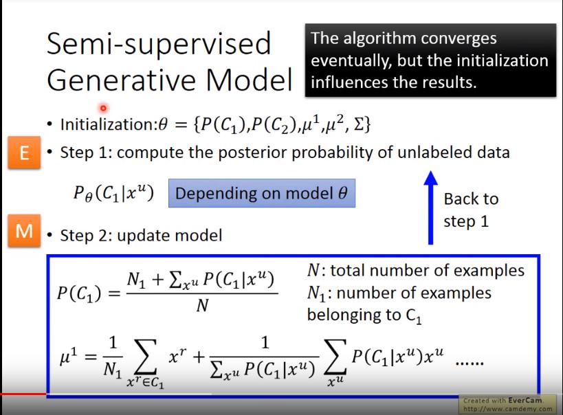
• Initialization: 計算出每個Class的機率、平均數、變異數
• Step1(EM算法中的E): 計算每個unlabeled data屬於某個Class的機率
• Step2(EM算法中的M): 更新model
  • 式1：融合labeled data和unlabeled data後，某個Class的機率
  • 式2：融合labeled data和unlabeled data後，某個Class的平均數

Why

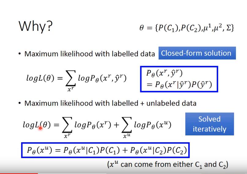
• Maximum likelihood with labeled data

  • 以 $\theta$ 的條件，能夠生成$(x^r,\hat y^r)$ 的機率
  • $logL(\theta)=\sum_\limits{x^r}logP_\theta(x^r,\hat y^r)$

• Maximum likelihood with labeled + unlabeled data

  • $log L(\theta)=\sum_\limits{x^r}log P_\theta(x^r,\hat y^r) + \sum_\limits{x^u}logP_\theta(x^u)$ (slide有誤)

Low-density separation

• 非黑即白
• 兩個Class之間會有一個很明顯的鴻溝

Self-training

1. 現有unlabeled data與labeled data
2. 使用labeled data 訓練出一個模型
3. 使用這個模型去predict unlabeled data
4. 選取某些預測好的unlabeled data及預測出來的pseudo label加入labeled data
5. 將擴充後的labeled data再丟進模型裡訓練

• regression通常不會使用這個方法
• Hard label(0 or 1) v.s. Soft label(Prob.)
  • 用hard label才有用
  • 前面介紹的 semi-supervised generative model 使用的是 soft label
  • 前面的generative model是使用soft label

Entropy-based Regularization

• 在unlabeled data中預測出來的class越集中越好
• $E(y^u) = -\sum_{m=1}^5 y_m^u ln(y_m^u)$ 越小(接近0)越好
• Lost Function: $L = \sum_\limits{x^r}C(y^r,\hat y^r)+\lambda\sum_\limits{x^u}E(y^u)$
  • 前項是原本的Loss，後面是unalbeled data的entropy，$\lambda$為自行決定的對unlabeled data entropy的懲罰係數

Semi-supervised SVM

• 窮舉所有unlabeled data的所有Class可能性
  • 使得SVM結果error最小，並且margin最大
  • 但不可能窮舉，因此一次先改一筆unlabeled data，看能不能讓 objective function(?)變大，變大就這樣改

Smoothness Assumption

假設

• 近朱者赤，近墨者黑
• x is not uniform (不平均)
• 若x1和x2之間的空間，資料點非常密集，則y1和y2會相同

實現

Cluster and then Label

- 需要有很好的方法來做clustering
- 圖片先使用 deep autoencoder抽feature，再做clustering會比較work

Graph-based Approach

- 建造graph來描述所有data point
- 建造時必須以high density path來連接，否則就算data point之間距離相近也不能做連接
- 必須自己定義graph如何建造
- 建造Graph
    1. 先定義similarity function {% math %}s(x^i,x^j){% endmath %}
    2. Add edge:
        - KNN: 將每個data尋找最相近的前K個鄰居連起來
        - e-Neighborhood: 將每個data尋找所有足夠相似(設定threshold)的其他point連起來
    3. 定義ㄧ個 Edge weight 使之和 {% math %}s(x^i,x^j){% endmath %} 成正比
        - **Gaussian Radial Basis Function(RBF)**較有用
            - {% math %}s(x^i,x^j)=exp(-\gamma |x^i-x^j|^2){% endmath %}
- 要使用Graph-based Approach必須確保data夠多，否則在graph斷掉的情況下，label沒辦法傳遞出去
- 定義 label smoothness
    - {% math %}S = \frac{1}{2}\sum_{i,j}w_{i,j}(y^i-y^j)^2 = y^TLy{% endmath %} 越小越好
        - i,j為相連的兩點
        - {% math %}w_{i,j}{% endmath %} 代表edge的weight，越大代表i,j兩點**離越近**
        - y是(R+U)維向量，{% math %}y=[...y^i...y^j...]^T{% endmath %}
        - L(**Graph Laplacian**)是(R+U)*(R+U)的matrix，{% math %}L=D-W{% endmath %}
            - W是所有點之間的 connection weight matrix
            - D是W矩陣的所有列總和，放在diagonal的位置
    - 因此在Loss Function加入一項 smoothness: {% math %}\lambda S{% endmath %}
        - {% math %}L=\sum_\limits{x^r}C(y^r,\hat y^r)+\lambda S{% endmath %}
        - 若是deep network，不一定要把 smoothness 放在output的地方，可以放在任何embedding layer

Better Representation

- 去蕪存菁，化繁為簡
- **Unsupervised Learning(Lec 15?)** 會詳談
- find the latent factors(usually simpler) behind the observation